Open this tutorial in Google Colab

Template fitting

Template fitting method calculates the amplitude, phase and zero point variation of a modulated time series by fitting a template defined by using the Fourier solution of the complete data set with the main pulsation frequency and its 𝑛 harmonics.

The method works as follows:

• First, using seismolab.fourier, it calculates a Lomb-Scargle spectrum and derives the frequency of the main peak in the spectrum,

• It also derives the harmonics of the main peak,

• Then, creates a template using this series of Fourier harmonics,

• Splits the light curve into overlapping chunks; the lengths are specified proportion to the main period,

• And finally fits the template to each chunk to yield the amplitude, phase and zero point at each time step.

Note: this method yields the variation of the global parameters; not the individual Fourier amplitudes and phase.

How to use

from seismolab.template import TemplateFitter

import numpy as np
import matplotlib.pyplot as plt
import pandas as pd

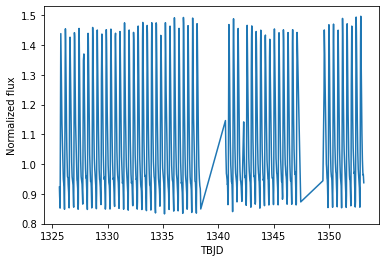
We load as an example the Blazhko modulated light curve of T Men from TESS Sector 1.

lc = pd.read_csv("https://mast.stsci.edu/api/v0.1/Download/file/?uri=mast:HLSP/qlp/s0001/0000/0000/4041/2372/hlsp_qlp_tess_ffi_s0001-0000000040412372_tess_v01_llc.txt")

# Store results in separate arrays for clarity
time       = lc.iloc[:,0]
brightness = lc.iloc[:,1]
brightness_error = np.ones_like(time)*0.01

plt.plot(time, brightness)
plt.xlabel("TBJD")
plt.ylabel("Normalized flux")
plt.show()

Performing a template fitting

We initialize the TemplateFitter by passing the light curve. Passing the measurement errors is optional, but without it the estimated errors will be unrealistic!

fitter = TemplateFitter(time, brightness, brightness_error)

The template fitting is done by calling fit.

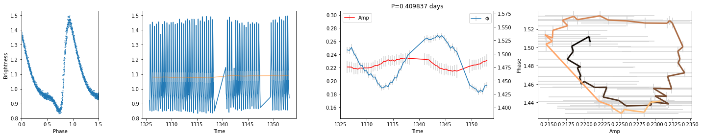
times, amp, amperr, phase, phaseerr, zp, zperr = fitter.fit(plotting=True,scale='flux')

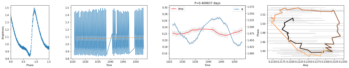
The results and its errors are stored in seven arrays:

• times is the equidistant time steps,

• amp & amperr are the temporal variation of the amplitude of the template and its uncertainty,

• phase & phaseerr are the temporal variation of the phase of the template and its uncertainty,

• zp & zperr are the temporal variation of the zero point of the template and its uncertainty.

All available options are described below:

times, amp, amperr, phase, phaseerr, zp, zperr = fitter.fit(
        span = 3,                    # Number of (pulsation) cycles to be fitted
        step = 1,                    # Steps in number of (pulsation) cycles
        error_estimation='analytic', # Can be `analytic` or `montecarlo`

        maxharmonics = 10,       # Max number of Fourier harmonics to be used in the template
        minimum_frequency=None,
        maximum_frequency=None,  # Overwrites nyquist_factor!
        nyquist_factor=1,        # The multiple of the average nyquist frequency
        samples_per_peak=100,    # Oversampling factor in Lomb-Scargle spectrum calculation
        kind='sin',              # Function type: `sin` or `cos`

        plotting=True,           # Show results
        scale='flux',            # Light curve scale, `mag` or `flux`
        saveplot=False,          # Save the plot as file
        saveresult=False,        # Save result as txt file
        filename = 'mystar',     # Filename without extension
        showerrorbar=True,       # Show errorbars in plots

        smoothness_factor=0.5,   # Smooth the curves by a Gaussian (0: None, 1-: strong smoothing)
        duty_cycle=0.6,          # Skip cycles if duty cycle is lower than this value (between 0-1)

        best_freq=None,          # Use this frequency for the basis of the Fourier harmonics
                                 # This option overwrites the automatic Lomb-Scargle frequency search

        debug=False              # Verbose output
    )

Constructing the modulated template light curve

To visualize the modulation of the template curve, it is suggested to calculate a well-sampled modulate curve first. To do, the steps in number of (pulsation) cycles is reduced, i.e. the sampling grid is refined.

times, amp, amperr, phase, phaseerr, zp, zperr = fitter.fit(
        span = 3,                    # Number of (pulsation) cycles to be fitted
        step = 0.01,                 # Steps in number of (pulsation) cycles
    )

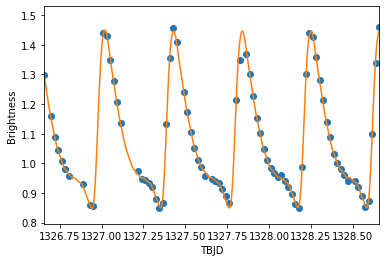
Then the well-sampled modulated template curve is constructed.

template = fitter.get_lc_model()

plt.plot( time, brightness,'o' )
plt.plot( times, template )
plt.xlim(time.min()+1,time.min()+3)
plt.xlabel("TBJD")
plt.ylabel("Brightness")
plt.show()

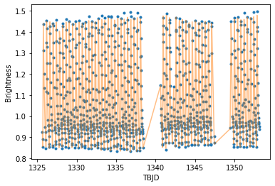
Resampling the template curve

Since the modulated template curve is sampled on a uniform grid, it is ought to be resampled at the time steps of the original light curve to e.g. get the residual light curve.

The resampled template curve can be easily constracted using an interpolation method.

template = fitter.get_lc_model_interp(kind='slinear')

plt.plot(time,brightness,'.')
plt.plot(time,template,alpha=0.5 )
plt.xlabel("TBJD")
plt.ylabel("Brightness")
plt.show()

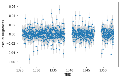
This template curve can be subtracted from the original light curve.

residual = brightness - template

plt.errorbar(time, residual, brightness_error, fmt='.', ecolor='lightgray' )
plt.xlabel("TBJD")
plt.ylabel("Residual brightness")
plt.show()

Comparing the spectra

To see the effect of subtracting the modulted template curve from the original light curve, one way is to compare the Fourier spectra of these data sets. Here, we also compare the results to the residual light curve, which is obtained by subtracting the sum of Fourier harmonics from the original observations.

from astropy.timeseries import LombScargle
from seismolab.fourier import MultiHarmonicFitter

Using the seismolab.fourier a series of Fourier harmonics are fitted and subtracted.

fourier = MultiHarmonicFitter(time,brightness)

pfit,perr = fourier.fit_harmonics(maxharmonics=100)

time, resbrightness, resbrightness_error = fourier.get_residual()

The Lomb-Scargle spectrum of each light curve is calculated.

lsf,lsp = LombScargle(time,brightness).autopower(nyquist_factor=1,
                                                 normalization='psd')
lsp_res      = LombScargle(time,resbrightness).power(lsf,normalization='psd')
lsp_template = LombScargle(time,residual).power(lsf,normalization='psd')

And transform to Fourier-like spectra.

lsp          = 2*np.sqrt(lsp/len(time))
lsp_res      = 2*np.sqrt(lsp_res/len(time))
lsp_template = 2*np.sqrt(lsp_template/len(time))

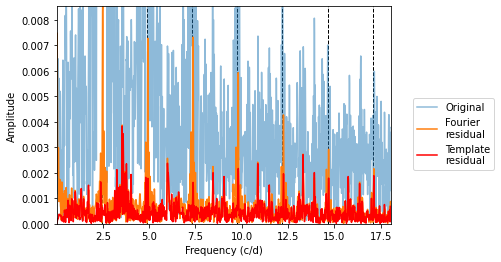
Comapring the three spectra, it can be seen that the side lobes (orange) of main peak and its harmonics (black dashed) of the original spectrum (blue) are suppresed in the template residual spectrum (red). However, the other, additional peaks are kept untouched.

plt.plot(lsf,lsp,alpha=0.5,label='Original')
plt.plot(lsf,lsp_res,label='Fourier\nresidual')
plt.plot(lsf,lsp_template,'r',label='Template\nresidual')

plt.xlim(lsf.min(),lsf.max())
plt.ylim(0,lsp_res.max())

for ii in range(1,10):
    plt.axvline( ii*pfit[0], c='k',zorder=0,lw=1.,ls='--')

plt.xlabel('Frequency (c/d)')
plt.ylabel('Amplitude')
plt.legend(bbox_to_anchor=(1.05,0,0,0.6))
plt.show()