![]()
Open this tutorial in Google Colab
Fourier
The Fourier module offers tools to calculate Fourier spectrum, extract the individual frequencies from the multiperiodic content of time series, to perform multiple-frequency fits and to derive Fourier parameters (see e.g. Simon & Lee 1981, ApJ, 248, 291).
It has three main options:
The
Fourieris designed to calculate the classic Fourier spectrum and the spectral window of a light curve.The
MultiHarmonicFitteris used to extract the parameters of the main frequency with the highest peak in the spectrum and its harmonics and to simultaneously fit those Fourier components to a time series. The derived components are the base of the Fourier parameter calculations.The
MultiFrequencyFitterextracts the parameters of all frequency components above a given threshold with pre-whitening steps in decreasing amplitude order.
Choosing the type of Fourier series
The Fourier series fit can be done via two ways. Fitting \(sine\) or \(cosine\) functions:
where \(A_i\) is the semi-amplitude, \(f_i\) is the frequency and \(\phi_i\) is the phase of the given component. The constant is the zero point of the light curve.
Note: This is optional in the code. Use the keyword kind='sin' or kind='cos' to select one. The default is sine.
The code first finds the frequency with the highest peak in the spectrum and after that does a consequtive pre-whitening with the integer multiples of that frequency. Thus, if we want to calculate the Fourier parameters of e.g. the second overtone, we have to put constraints on the frequency range to be checked i.e. minimum_frequency and maximum_frequency must be defined. Otherwise the highest peak in the spectrum will be considered.
Note: If due to sparse sampling the Nyquist limit is low (e.g. in case of ground-based observations), set maximum_frequency to overwrite the default Nyquist limit.
Fourier parameters
After fitting at least 3 frequencies, the Fourier parameters can be calculated as
which values depend on the chosen function (sine or cosine), the physical units (flux or mag) and the passband as well. The more the harmonics, the more accurate the results.
Note: To get all harmonics, set nfreq to a very large number (e.g. 9999), which case the number of harmonincs will be limited by the signal-to-noise ratio.
Error estimation
Errors are estimated analytically by default using the formulae of Breger (1999, A&A, 349, 225):
However, errors can also be estimated in two other, more reliable ways.
Set
error_estimationto'bootstrap'to enable the bootstrap method.Or set
error_estimationto'montecarlo'to enable the monte carlo method.
Both methods generate new light curves ntry times and fit each dataset induvidually. The results are collected and the parameter uncertenties are estimated from the distributions.
Bootstraping:
To generate new data sets the bootstrap method subsamples the light curve. The number of sampled points are controlled by the sample_size (= ratio between 0-1) parameter.
Monte Carlo sampling:
The monte carlo method generates light curves with the same number of points as the original number of points. Each brightness measurement is resampled from a Gaussian with mean equals to the original brightness and std equals to the noise. If light curves noise is not known, then it is estimated from the residual light curve.
To speed up the sampling process, the code can be run parallel via setting parallel to True. By deafult, all the CPU cores are used, but this can be limited by setting ncores.
Note: The resulted distributions and their correlations can be visualized by setting plotting to True. However, to decouple the frequencies from the phases the time points are constrained by
Thus, the absolute values of the plotted phases will differ from the returned ones. They are only used to estimate errors.
Noise calculation
In case of the MultiFrequencyFitter, the S/N ratio is calculated at each pre-whitening step and it is used as a stopping condition. To do so, the noise is calculated in a range around the given frequency using the residual spectrum. The range can be set by the user with the boxwidth keyword, then the noise is calculated as the mean of the spectrum in the range of:
How to use
[1]:
from seismolab.fourier import Fourier, MultiHarmonicFitter, MultiFrequencyFitter

import numpy as np
import matplotlib.pyplot as plt
import pandas as pd
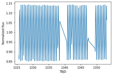
We load as an example the light curve of ST Pic from TESS Sector 1.
[2]:
lc = pd.read_csv("https://mast.stsci.edu/api/v0.1/Download/file/?uri=mast:HLSP/qlp/s0001/0000/0001/5016/6721/hlsp_qlp_tess_ffi_s0001-0000000150166721_tess_v01_llc.txt")

# Store results in separate arrays for clarity
time       = lc.iloc[:,0]
brightness = lc.iloc[:,1]
[3]:
plt.plot(time, brightness)
plt.xlabel("TBJD")
plt.ylabel("Normalized flux")
plt.show()
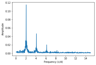
Calculating the classic Fourier spectrum
We initialize the Fourier by passing the light curve.
[4]:
FF = Fourier(time,brightness)
The Fourier spectrum is calculated with ``spectrum``.
[5]:
FFf, FFp = FF.spectrum(maximum_frequency=15, samples_per_peak=10)
[6]:
plt.plot(FFf, FFp)
plt.xlabel("Frequency (c/d)")
plt.ylabel("Amplitude")
plt.show()
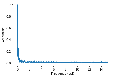
The spectral window can be used to filter alias peaks in the spectrum.
[7]:
swf,swp = FF.spectral_window(maximum_frequency=15)

plt.plot(swf,swp)
plt.xlabel("Frequency (c/d)")
plt.ylabel("Amplitude")
plt.show()
Extracting the main frequency and its harmonics
We initialize the MultiHarmonicFitter by passing the light curve. Passing the measurement errors is optional, but it strongly affects the results!
[8]:
fitter = MultiHarmonicFitter(time,brightness)

# The same can be done with measurement errors
#fitter = MultiHarmonicFitter(time,brightness,brightness_error)
Prewhitening with given number of harmonics are done via ``fit_harmonics``.
[9]:
pfit,perr = fitter.fit_harmonics(
    maxharmonics = 3,            # Set to e.g. 9999 to fit all harmonics
    sigma = 4,                   # S/N ratio above which a frequency is considered significant
    kind='sin',                  # Fourier series type, 'sin' or 'cos'

    minimum_frequency=None,
    maximum_frequency=20,        # Overwrites nyquist_factor!
    nyquist_factor=1,
    samples_per_peak=100,        # Oversampling factor in Lomb-Scargle spectrum calculation

    plotting = True,             # Show spectrum and phase curve
    scale='flux',                # Light curve scale, `mag` or `flux`

    error_estimation='analytic', # Method of the error estimation
    ntry=1000,                   # Number of samplings if method is NOT `analytic`
    sample_size=0.999,           # Subsample size if method is `bootstrap`
    parallel=True,               # Parallel sampling if method is NOT `analytic`
    ncores=-1,                   # Number of cores if method is NOT `analytic`

    best_freq=None               # Use this frequency for the basis of the Fourier harmonics
                                 # This option overwrites the automatic Lomb-Scargle frequency search
)

The results and its errors are stored in two arrays, in the following order:
the main frequency in cycle/days,
the amplitudes and phases of the main frequency and its harmonics,
the zero point.
These can be printed e.g. as follows:
[10]:
print('Freq = %.6f +/- %.6f' % (pfit[0], perr[0]) )

ncomponents = int((len(pfit)-1)/2)

for i in range(1, ncomponents + 1 ):
    print('A%d   = %.6f +/- %.6f' % (i, pfit[i],             perr[i]) )
    print('Phi%d = %.6f +/- %.6f' % (i, pfit[i+ncomponents], perr[i+ncomponents]) )

print('Zero point = %.2f +/- %.2f' % (pfit[-1], perr[-1]) )
Freq = 2.058955 +/- 0.000052
A1   = 0.115327 +/- 0.000299
Phi1 = 2.026532 +/- 0.000412
A2   = 0.046095 +/- 0.000299
Phi2 = 3.995322 +/- 0.001031
A3   = 0.019665 +/- 0.000299
Phi3 = 6.163608 +/- 0.002416
Zero point = 1.00 +/- 0.03
The Fourier parameters can be calculated as follows.
The results are uncertainties. The first two returned values are the main frequency and period with their errors, in cycle/days and days, respectively. The last two values are lists containing the \(R_{n1}\), \(\Phi_{n1}\) Fourier parameters.
[11]:
freq, period, Rn1, Phin1 = fitter.get_fourier_parameters()
[12]:
print('Freq   = %.6f +/- %.6f' % (freq.n,   freq.s) )
print('Period = %.6f +/- %.6f'%  (period.n, period.s) )

for i,(Rn,Phin) in enumerate(zip(Rn1,Phin1)):
    print('R%d1   = %.3f +/- %.3f' % ((i+2), Rn.n,   Rn.s) )
    print('Phi%d1 = %.3f +/- %.3f' % ((i+2), Phin.n, Phin.s) )
Freq   = 2.058955 +/- 0.000052
Period = 0.485683 +/- 0.000012
R21   = 0.400 +/- 0.003
Phi21 = 6.225 +/- 0.001
R31   = 0.171 +/- 0.003
Phi31 = 0.084 +/- 0.003
The fitted sum of Fourier harmonincs can be reconstructed and visualized.
[13]:
tmodel = np.linspace(time.min(),time.max(),10000)

lcmodel = fitter.lc_model(tmodel,*pfit)
[14]:
plt.scatter(time,brightness,c='k')
plt.plot(tmodel,lcmodel)
plt.xlim(time.min(),time.min()+2)
plt.gca().invert_yaxis()
plt.xlabel("Time")
plt.ylabel("Brightness")
plt.show()

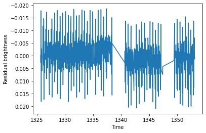
The residual light curve can also be easily constructed.
[15]:
time, resbrightness, resyerr = fitter.get_residual()

plt.plot(time,resbrightness)
plt.gca().invert_yaxis()
plt.xlabel("Time")
plt.ylabel("Residual brightness")
plt.show()
Extracting all frequencies
We initialize the MultiFrequencyFitter by passing the light curve. Passing the measurement errors is optional, but it strongly affects the results!
[16]:
fitter = MultiFrequencyFitter(time,brightness)

# The same can be done with measurement errors
#fitter = MultiFrequencyFitter(time,brightness,brightness_error)
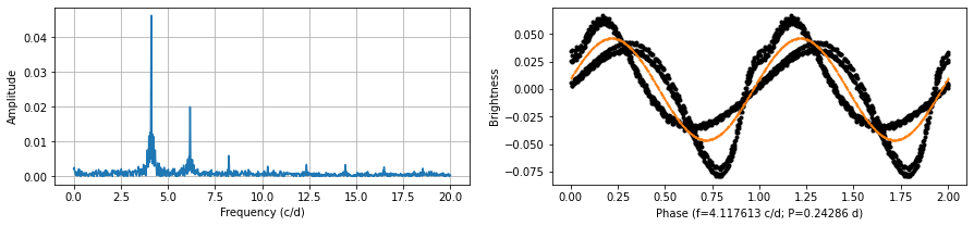
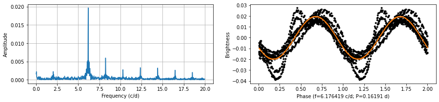
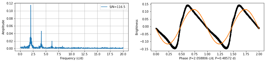
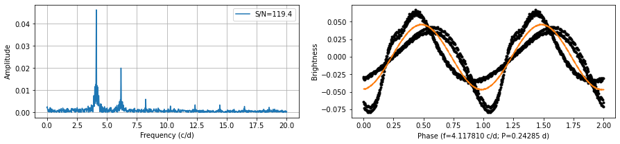
Prewhitening with given number of frequencies are done via ``fit_freqs``.
[17]:
pfit,perr = fitter.fit_freqs(
maxfreqs = 3, # Set to e.g. 9999 to get all frequencies
sigma = 4, # S/N ratio above which a frequency is considered significant
boxwidth = 1, # The frequency range to be used to calculate noise in the residual spectrum
kind='sin', # Fourier series type, 'sin' or 'cos'
minimum_frequency=None,
maximum_frequency=20, # Overwrites nyquist_factor!
nyquist_factor=1,
samples_per_peak=100, # Oversampling factor in Lomb-Scargle spectrum calculation
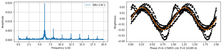
plotting = True, # Show spectrum and phase curve
scale='flux', # Light curve scale, `mag` or `flux`
error_estimation='analytic', # Method of the error estimation
ntry=1000, # Number of samplings if method is NOT `analytic`
sample_size=0.999, # Subsample size if method is `bootstrap`
parallel=True, # Parallel sampling if method is NOT `analytic`
ncores=-1 # Number of cores if method is NOT `analytic`
)
The results and its errors are stored in two arrays, in the following order:
the frequencies in cycle/days,
the amplitudes and phases,
the zero point.
These can be printed e.g. as follows:
[18]:
ncomponents = int((len(pfit)-1)//3)

for i in range(ncomponents):
    print('f%d   = %.6f %.6f' % ((i+1),  pfit[i],               perr[i]) )
    print('A%d   = %.6f %.6f' % ((i+1),  pfit[i+ncomponents],   perr[i+ncomponents]) )
    print('Phi%d = %.6f %.6f' % ((i+1), pfit[i+2*ncomponents], perr[i+2*ncomponents]) )

print('Zero point = %.3f %.3f' % (pfit[-1], perr[-1]) )
f1   = 2.058971 0.000052
A1   = 0.115325 0.000299
Phi1 = 1.892002 0.000412
f2   = 4.117866 0.000130
A2   = 0.046097 0.000299
Phi2 = 4.363133 0.001031
f3   = 6.176849 0.000305
A3   = 0.019664 0.000299
Phi3 = 0.010598 0.002416
Zero point = 0.998 0.032
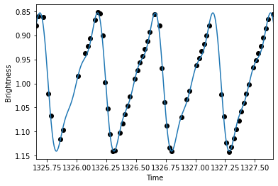
The fitted sum of all derived frequncies can be reconstructed and visualized.
[19]:
tmodel = np.linspace(time.min(),time.max(),10000)

lcmodel = fitter.lc_model(tmodel,*pfit)
[20]:
plt.scatter(time,brightness,c='k')
plt.plot(tmodel,lcmodel)
plt.xlim(time.min(),time.min()+2)
plt.gca().invert_yaxis()
plt.xlabel("Time")
plt.ylabel("Brightness")
plt.show()
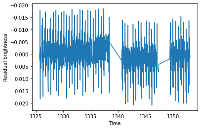
The residual light curve can also be easily constructed.
[21]:
time, resbrightness, resyerr = fitter.get_residual()

plt.plot(time,resbrightness)
plt.gca().invert_yaxis()
plt.xlabel("Time")
plt.ylabel("Residual brightness")
plt.show()